Finite Element Analysis: Stress Concentrations and Convergence Studies

Context

This work comes from two assignments completed during my structural engineering coursework at UC San Diego. The class started with analytical hand methods, working through calculus and the differential equations that govern linear elasticity, before moving into numerical implementation in Abaqus. That sequencing trained a specific kind of intellectual discipline: a finite element model produces a number, and that number can be wrong in ways that look right.

Both projects ask where stress concentrates in a part with geometric discontinuities. Both require demonstrating that the reported maximum is actually the maximum the model can resolve. The first project covers the analytical setup and mesh study. The second extends the same methodology into Richardson extrapolation and formal error analysis.

The Two Problems

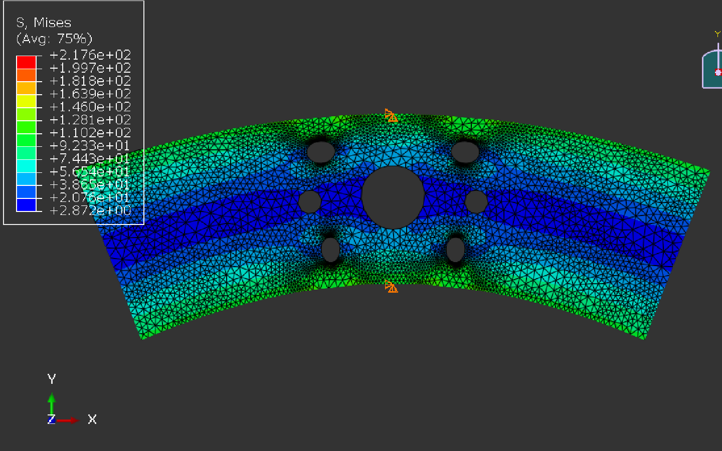
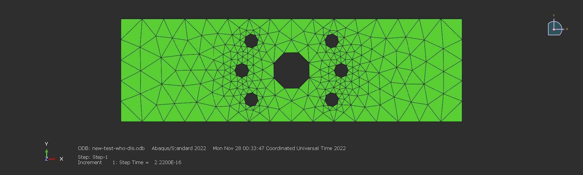
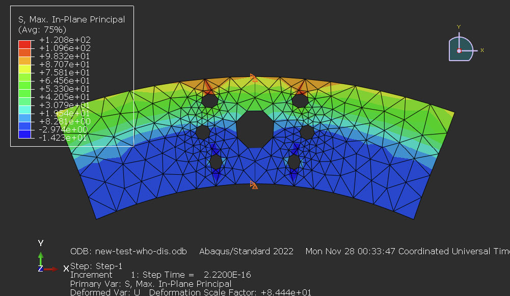
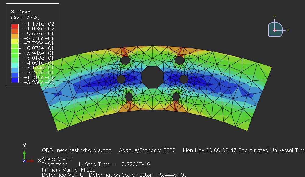
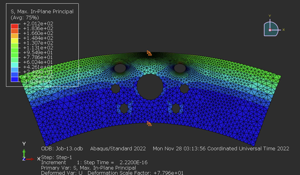
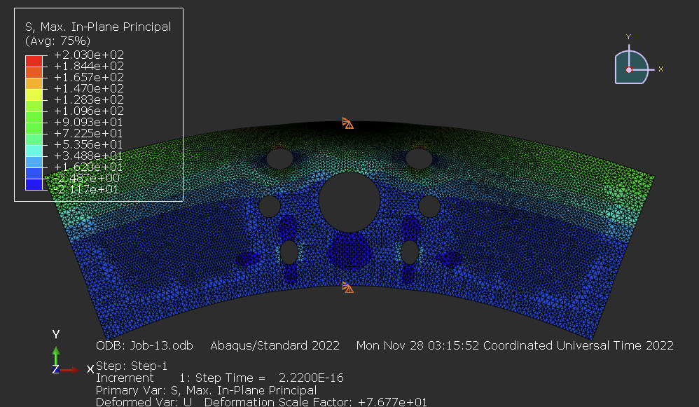
The first assignment placed a 2.5 mm aluminum slab with seven circular cutouts under self-equilibrated bending traction of 100 MPa at the extreme fibers. The geometry includes one central cutout (6.73 mm radius) surrounded by six smaller cutouts (2.5 mm radius each). The task was to identify the location and magnitude of the maximum tensile stress, then to verify that finding through mesh refinement.

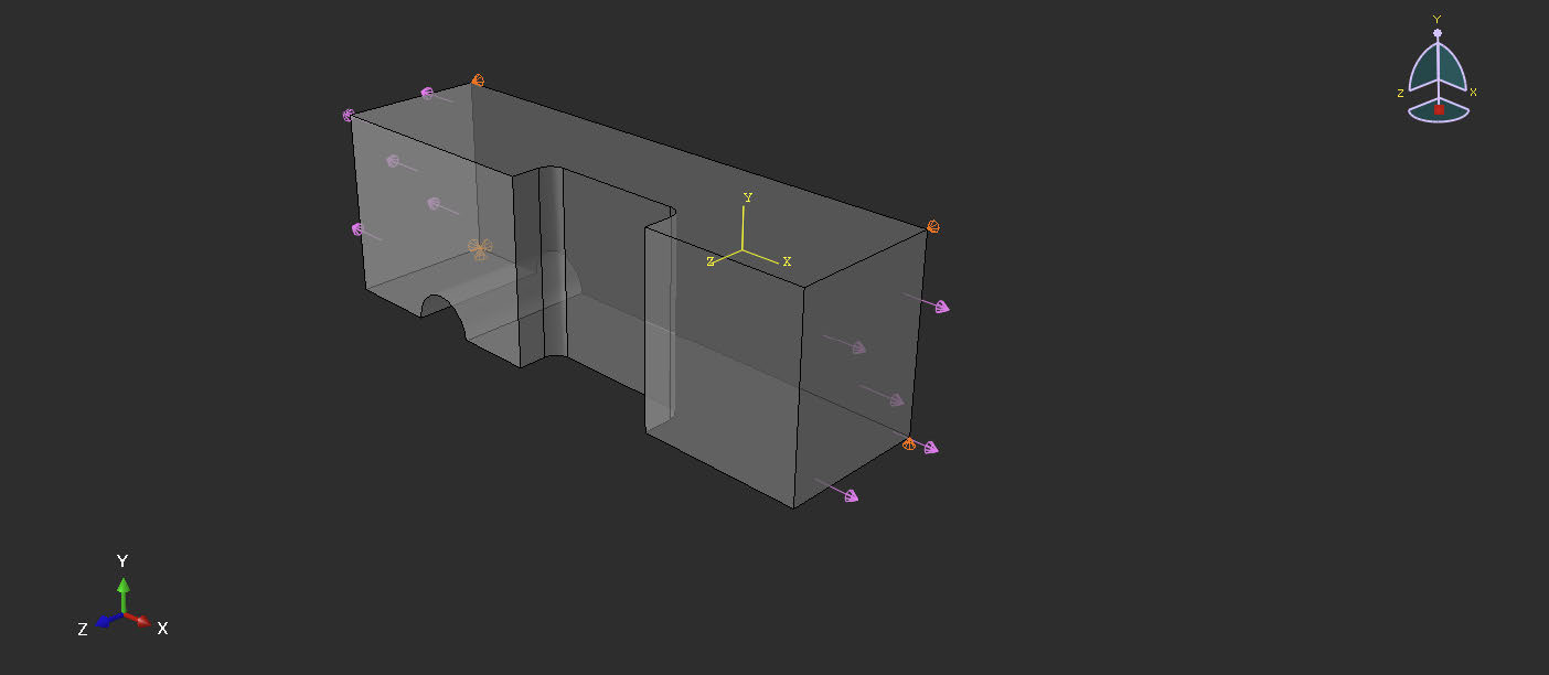
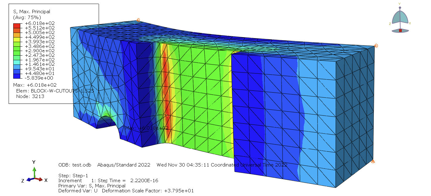
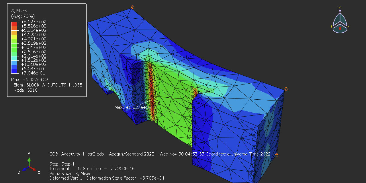
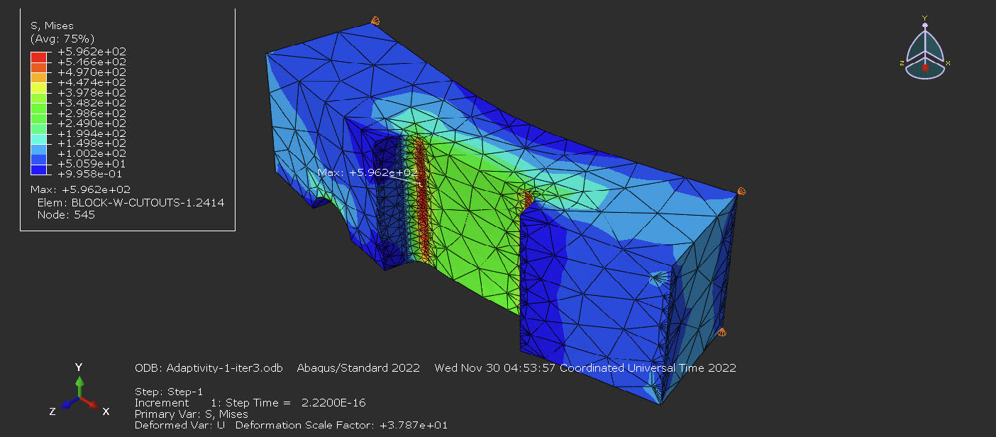
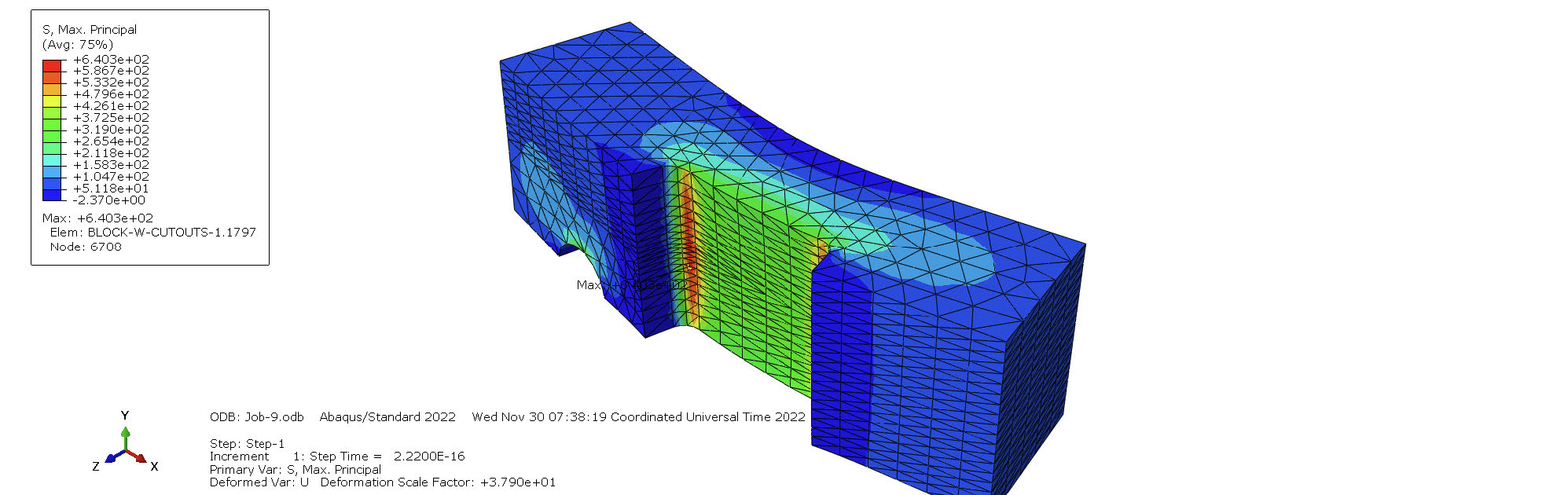
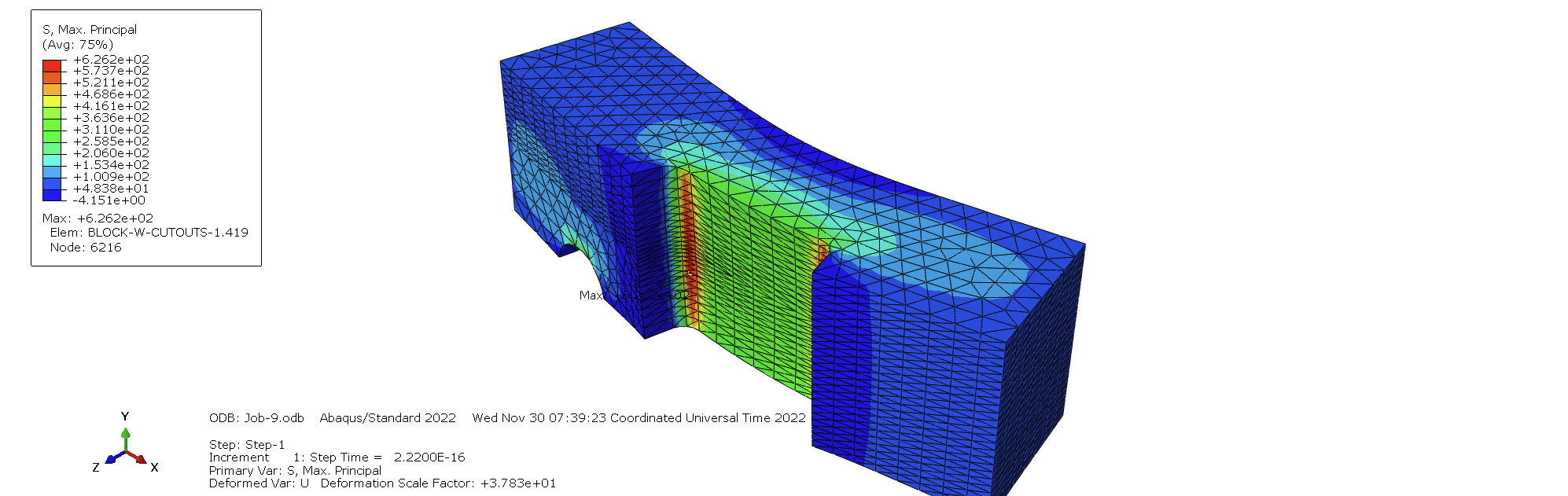
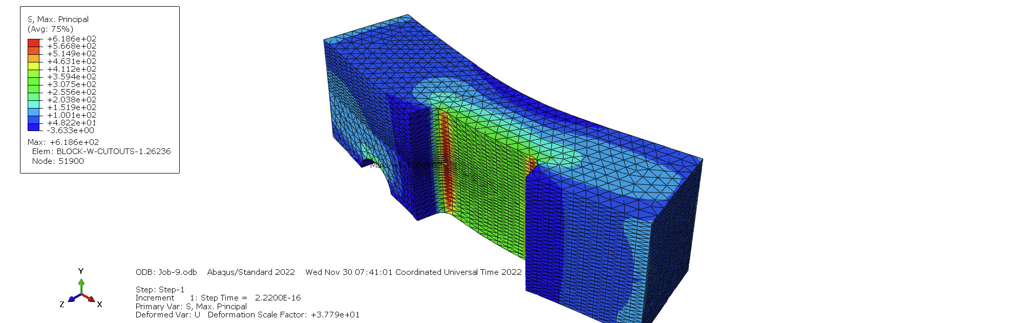
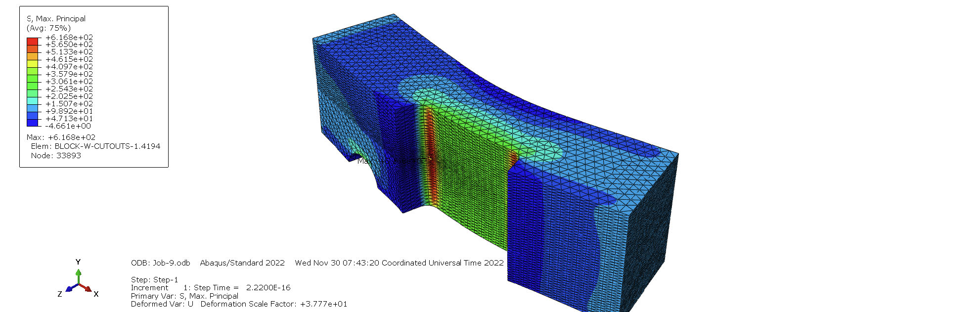
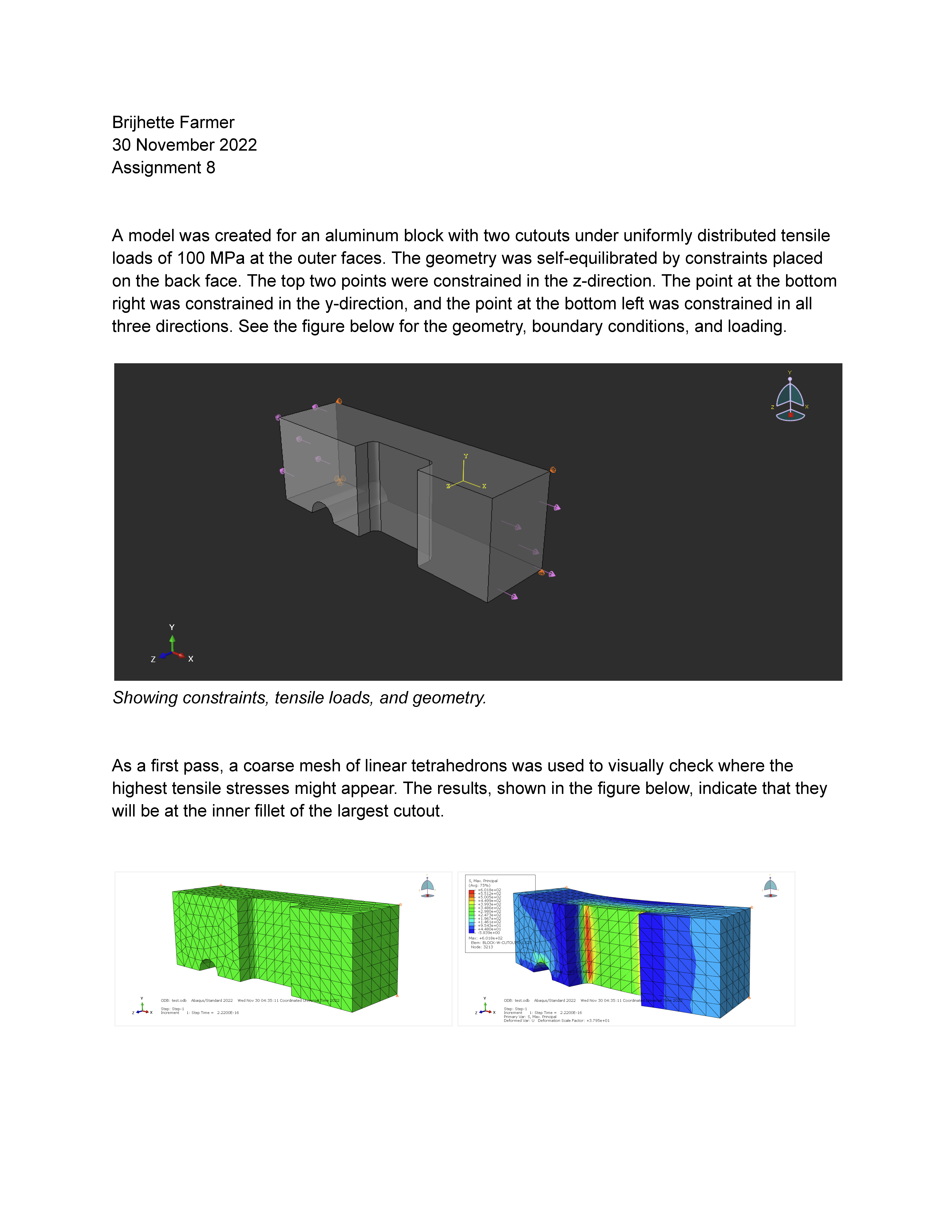
The second assignment used a three-dimensional aluminum block with two cutouts, loaded by uniform tensile tractions of 100 MPa on the outer faces. Constraints at the back face self-equilibrated the geometry. This part introduced fillet regions where stress concentration was visible from the first coarse mesh.

The hand calculations from earlier in the class anchored both. Working stress raisers by hand using classical Kirsch-style solutions teaches you the rough shape of the answer before software produces a precise-looking number. That preparation matters when a coarse mesh reports a value off by a factor of two and the result still looks plausible on screen.

Methodology

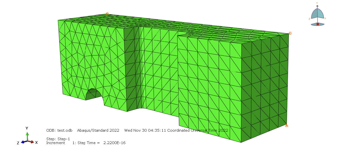
Each part was modeled through a progression of meshes. The first pass used a coarse, uniform mesh to establish the qualitative stress field and verify the model setup. From there, refinement happened through several mechanisms.

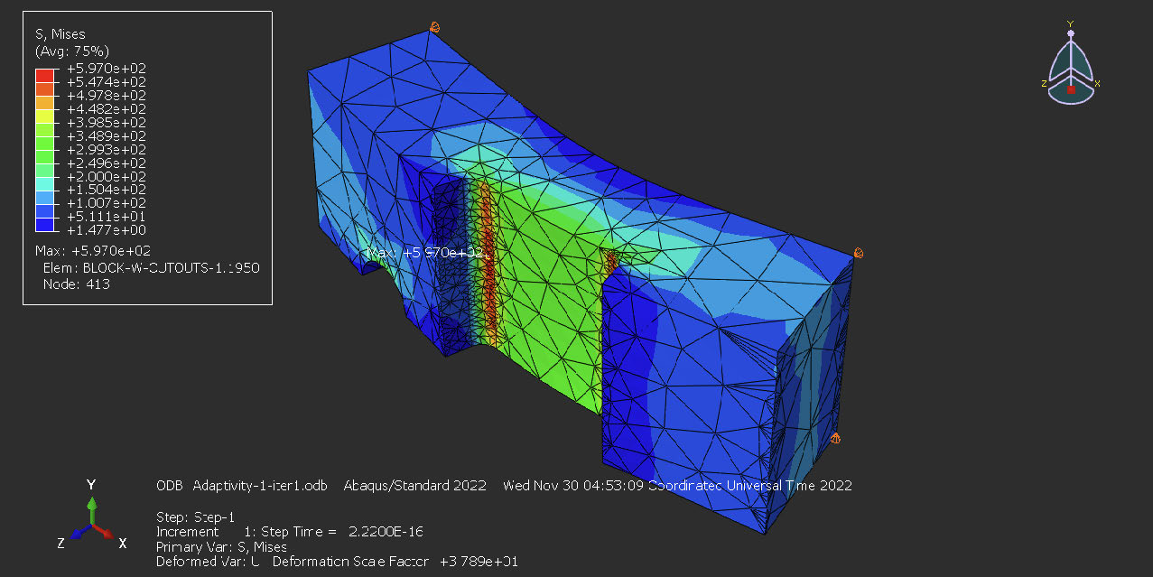
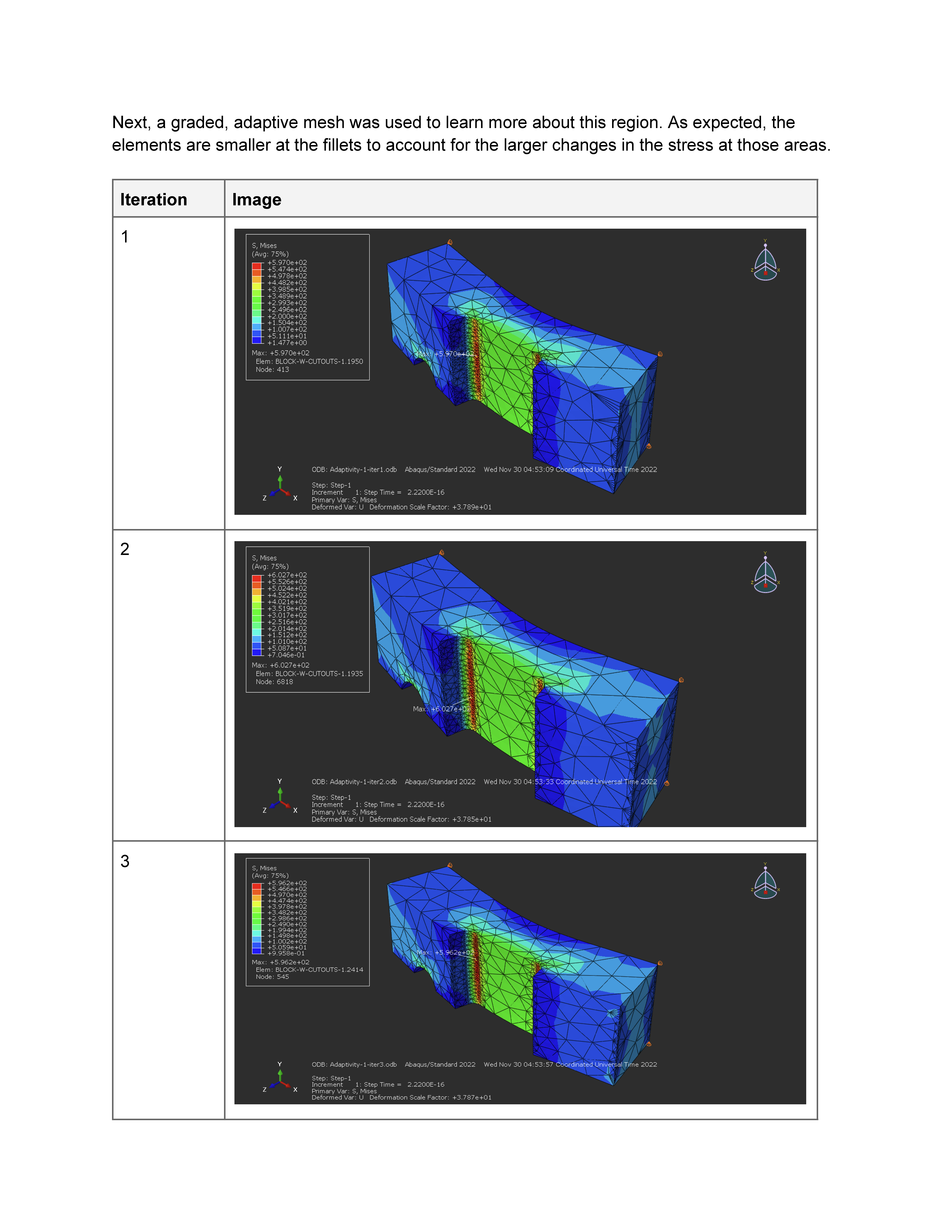
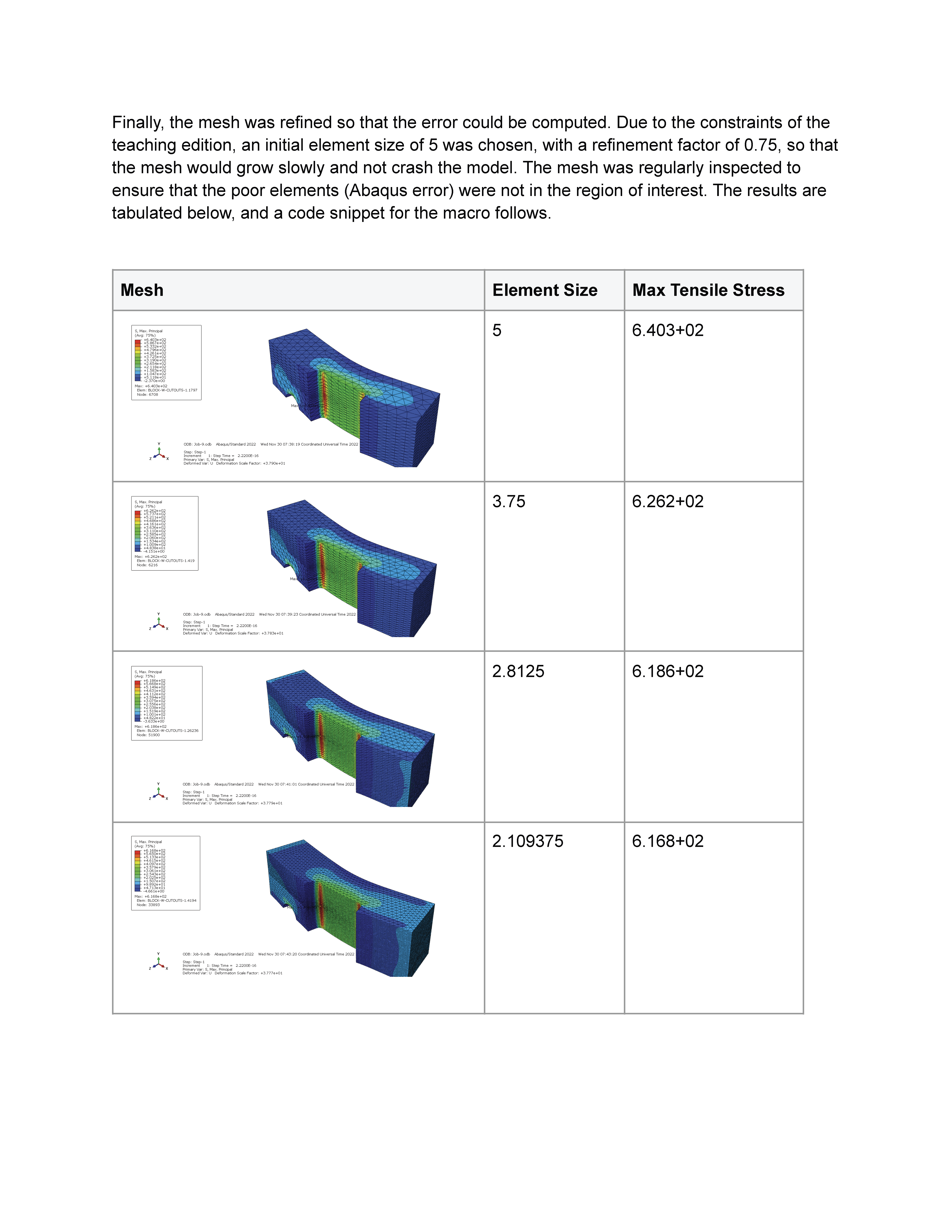
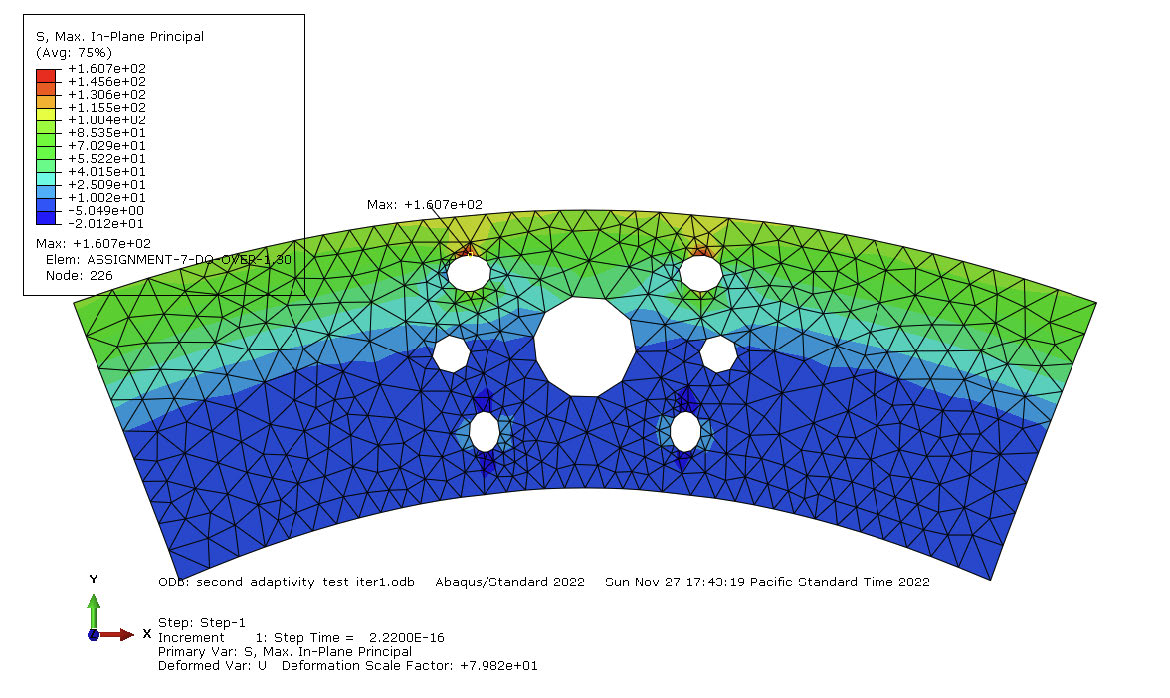
Local seeding placed smaller elements around the holes and fillets where stress gradients are steep. H-adaptivity, applied through Abaqus macros, allowed the software to refine elements based on solution error. For the second project, a Python macro looped through refinement iterations with a 0.75 scaling factor, generating four meshes at element sizes of 5, 3.75, 2.8125, and 2.109375.

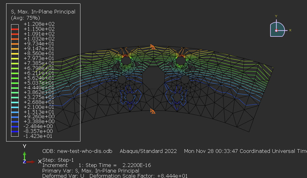
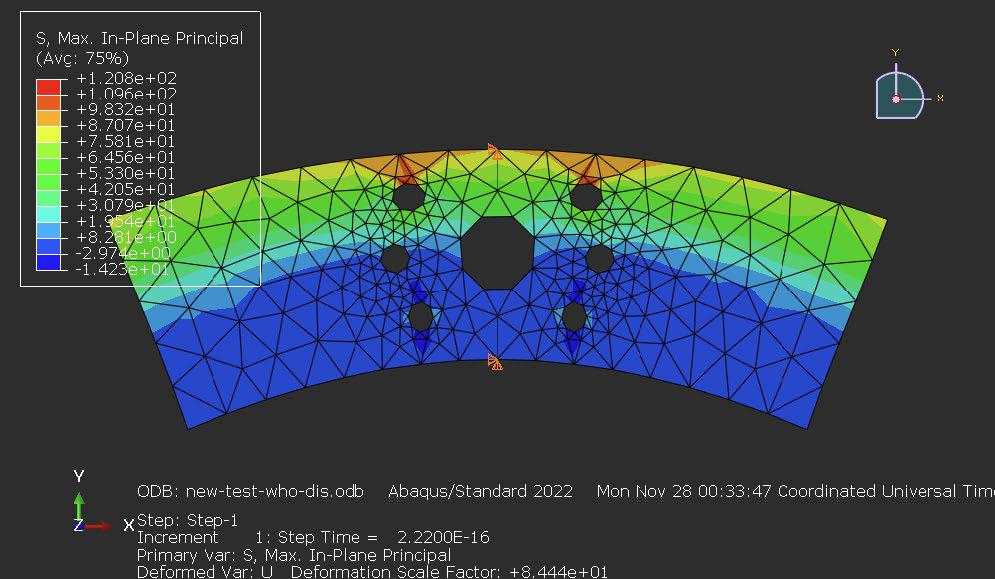
Two visualization choices were used to test whether the solution had converged. Banded contours show smoothed stress distributions. Isosurface contours expose discontinuities between elements. Toggling nodal averaging off in either view reveals where element-to-element jumps remain large, a signal that the mesh has not yet resolved the stress field in that region.

Richardson extrapolation provided the mathematical estimate of the true solution. With three computed values from successively finer meshes, the technique estimates both the converged value and the convergence rate. The last three meshes of the second assignment converged to 616.24 MPa with a convergence rate of 0.143.

Findings

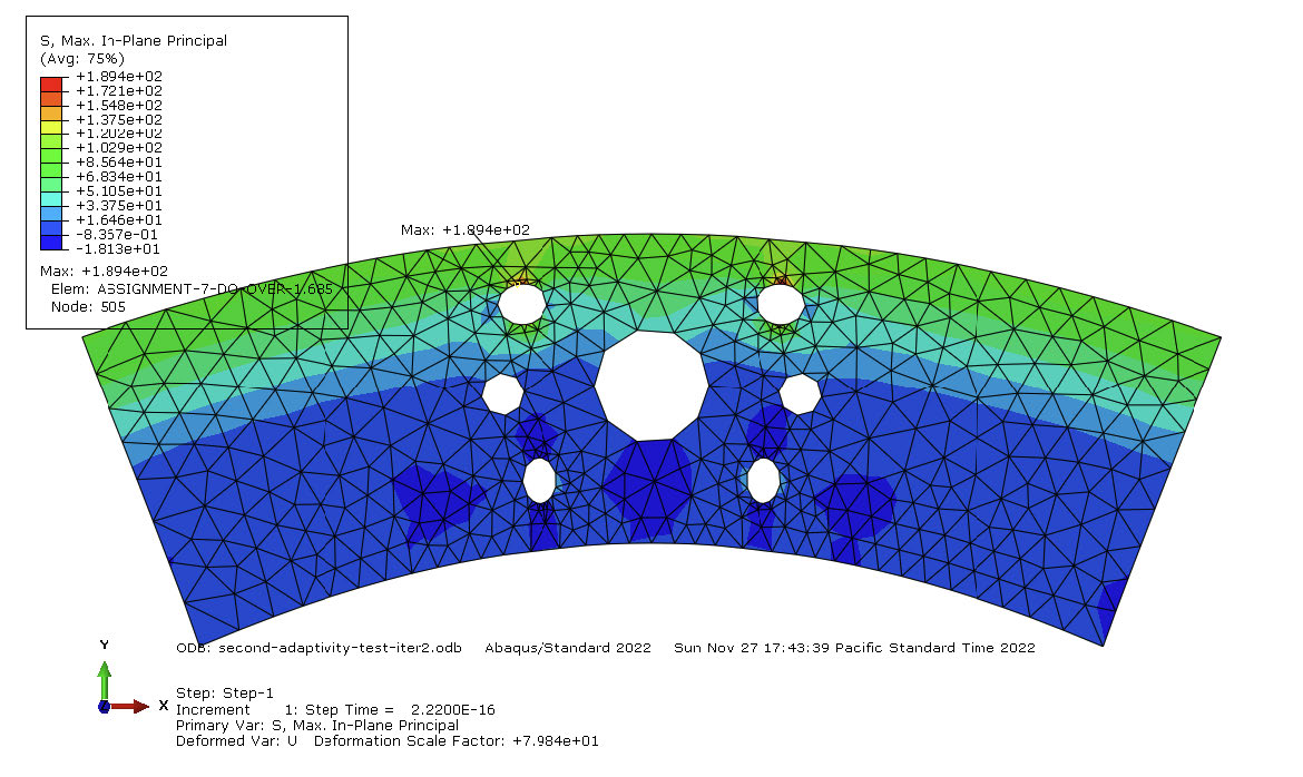
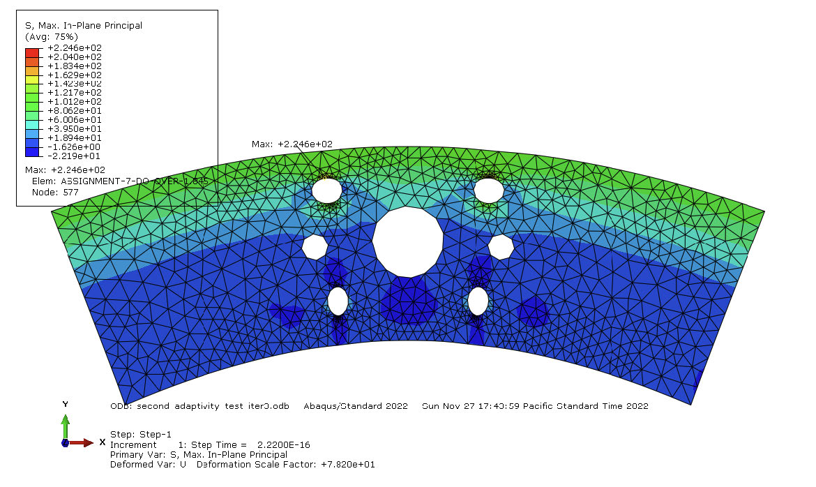
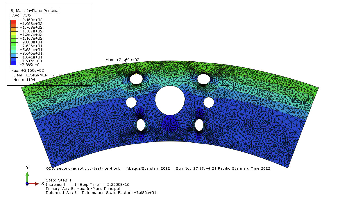
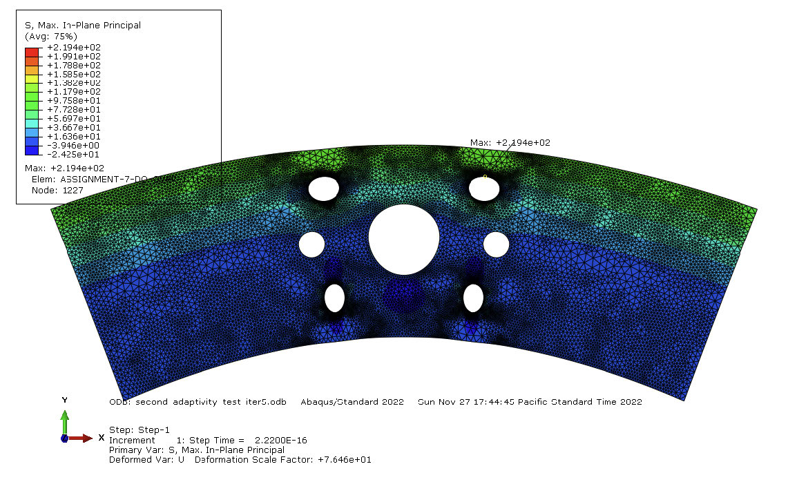
Initial estimates of maximum tensile stress on the aluminum slab were significantly low. The coarse mesh reported 1208 MPa. Through successive h-adaptive iterations, the value rose to 2194 MPa, an 82 percent change. That magnitude of correction makes the case for mesh study on its own.

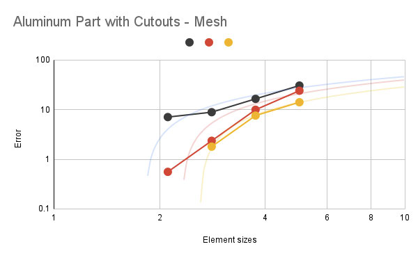
A cleaner demonstration came from the second assignment. The Richardson-extrapolated maximum tensile stress at the inner fillet of the larger cutout came in at 616.24 MPa, with errors decreasing in a way that produced a roughly straight line on a log-log plot of error against element size. This is what convergence looks like when the model is set up correctly.

Design Decisions

A few choices in this work are worth naming explicitly.

Adaptive meshing over uniform refinement. Refining everywhere wastes computation. The h-adaptive macro put elements where the solution gradient was largest, which is the only place mesh resolution actually changes the answer.

Nodal averaging used as a diagnostic. The default Abaqus view averages stresses across nodes, which produces visually smooth contours that can hide a poorly converged mesh. Turning averaging off was used to verify that adjacent elements were reporting compatible stresses in the regions of interest.

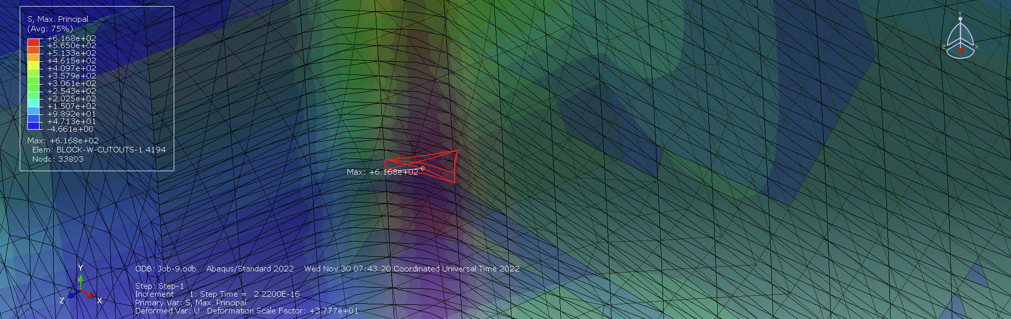
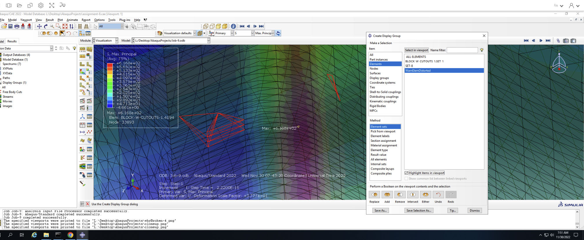
Element shape inspection in the convergence study. A refined mesh containing distorted elements gives worse results than a coarser mesh with well-shaped elements. The second assignment included a step that confirmed the poor-quality elements (flagged by Abaqus) sat outside the region of interest before the result was accepted.

Richardson extrapolation as a closing argument. A single number from a single mesh asks the reader to trust that the mesh was fine enough. Three numbers from a refinement sequence, plus an extrapolated true value and a convergence rate, let the reader see the argument.

Known Errata

The first assignment carries documented errors that I named at submission and preserve here.

The original model file corrupted during the assignment window. The remaining file used boundary conditions that were not what I would now apply. A simply supported configuration would have produced zero reactions, which was the cleaner answer to the boundary condition question. The reactions in the submitted work were nonzero and required additional explanation.

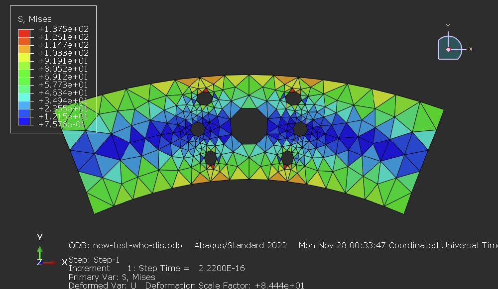
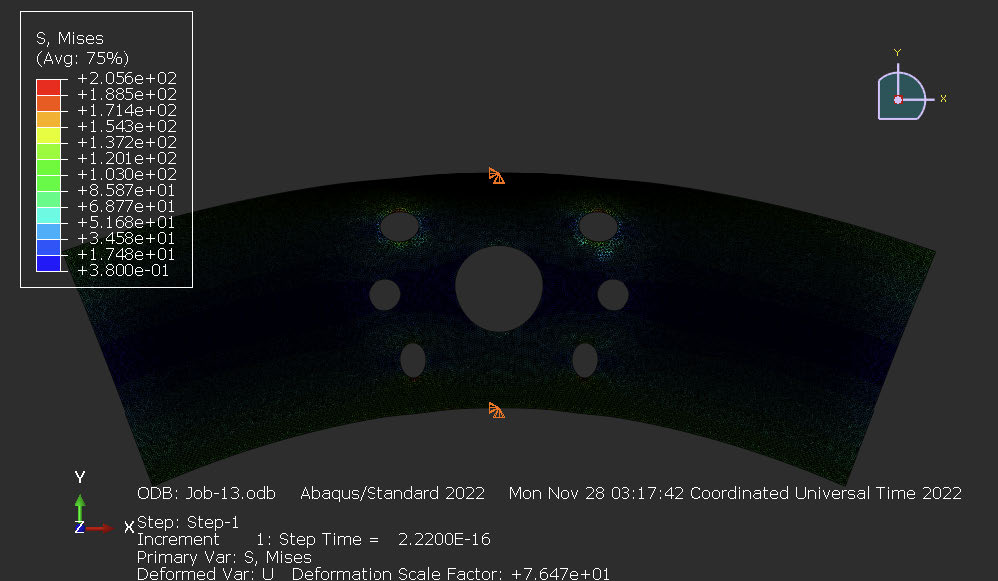
Several stress contour plots in the first assignment show Von Mises stress where the assignment asked for maximum in-plane principal stress. The mislabeling came from the corrupted model rebuild and could not be corrected in the submission window.

The local seed mesh in the first assignment refined toward the line of symmetry rather than only around the holes. This introduced a numerical singularity along the symmetry edge, which produced spurious stress values that were not part of the actual solution. The second assignment corrected this approach, refining only around the geometric features where stress concentration was physically expected.

Richardson extrapolation was carried out fully in the second assignment rather than the first. Both assignments asked for it. The first submission acknowledged that the methodology was demonstrated correctly in the second.

These errata matter because the discipline of finite element work depends on the reader being able to trust what is reported. Naming the failures preserves that trust.

Questions and Learnings

The methodology developed in these assignments covers mesh refinement, adaptive meshing, Richardson extrapolation, and error analysis. Together, these form the validation backbone of any structural simulation. For the disaster resilience work I am building toward, that matters in a specific way.

Damage prediction in seismic events depends on accurately resolving stress concentrations at geometric discontinuities and material transitions. Structural health monitoring systems rely on finite element models of buildings to interpret sensor data and assess damage state. Convergence studies are what transform a model from a calculation that produces numbers into an estimate with known confidence.

The questions this work generates for me now: how do these convergence techniques translate to nonlinear material behavior under dynamic loading, where the constitutive model itself introduces uncertainty? And what does it take to communicate the difference between a converged result and a validated prediction to a stakeholder making decisions about a building?

A structural engineer asks these questions before trusting a model. Answering them rigorously is what PhD programs in disaster resilience train researchers to do.

‍